Principal Component Analysis (PCA)
This analysis tool finds weighted combinations of variables that explain the variance between cases (rows) in the data set. This method ordinarily explains most of the variance using fewer weighted combinations of variables (principal components) than the number of original variables. It therefore accomplishes dimensionality reduction and also identifies the variables that contribute most to the overall variation in the data set.
The PCA tool requires that the data set have a single-column candidate key (which must be a text variable). If there are multiple candidate keys in the data set, the dialog will prompt for the one to use; if there is only one candidate key, it will be automatically selected. If the data set contains a numeric candidate key, a corresponding text variable can be created using the Table/Recode data menu item.

The PCA dialog prompts for:
Whether to carry out this analysis for all data in the data table or only for the subset that is selected on the map and in the data table.
Whether to remove missing values from the data set by eliminating variables (columns) with missing values or by eliminating cases (rows) with missing values.
Whether to normalize the data for each variable by subtracting the mean and dividing by the standard deviation, producing Z scores for use by the analysis.
The candidate key column to use, if there is more than one.
Three or more variables from the list displayed at the left of the dialog.
After these values have been selected or changed, the PCA calculation will be carried out automatically and the results will be summarized in the tables and plots on the right side of the dialog.
Note that even if three or more variables are selected, removal of missing values by variable deletion may reduce the number of variables to fewer than three.
Results of the PCA analysis are shown in tables and plots, each on a separate tab. These are:
Scores–The coordinates of each sample along each of the newly-derived orthogonal axes represented by the principal components. This table has one row for each data row used for the PCA analysis, and one column for each principal component. The first column of the table contains the candidate key values for the data rows.
Loadings–The weights of the variables’ contributions to each principal component. This table has one row for each principal component and one column for each variable.
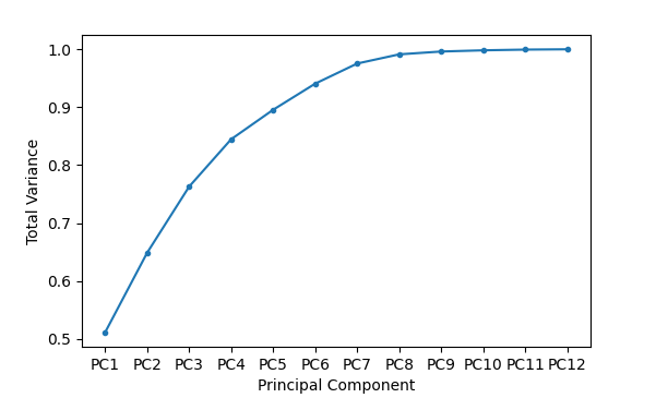
Explained variance–Principal components are constructed so that the first one explains most of the variance in the data set, the second one explains most of the remaining variance, and so forth. This table has one row for each principal component and three columns. The first column contains the variance, the second column contains the variance as a fraction of total variance, and the third column contains a running total of the fractional variance.
Scree plot–The scree plot shows the running sum of fractional variance against the principal component number. This is the same information that is in the Explained variance table, but in a visual form.
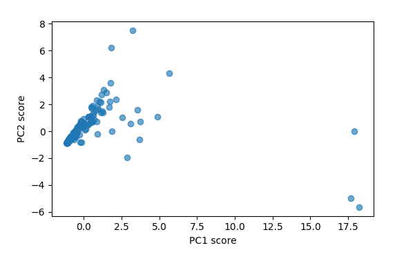
PC x PC plots–This tab will display a scatter plot of any two PCA scores. The plot is blank immediately after a PCA analysis is run. Principal components for the X and Y axes must be selected from the dropdown lists above the scatter plot. Hovering over a point on the scatter plot with the mouse will display the candidate key value for that point (or points if they are close together). The transparency (alpha value) of the points can be modified with the Alt-A keystroke.
The “Source Data” button at the bottom of the dialog will display a table of all selected data. The table can be saved using the Ctrl-S keystroke.
The “Add Columns” button at the bottom of the dialog is only active when the Scores table is displayed. This button will append the PCA scores for each data row to the data table. The names of the new data table columns will be “PC1”, “PC2”, etc., prefixed with additional text that can be used to distinguish different sets of PCA output. Mapdata will prompt for both the number of principal components to copy to the data table, and for the column prefix to use. The prefix will be separated from the rest of each column name with an underscore. The results of the PCA can then be used to select and highlight data rows, change map symbology, create data plots, or to carry out other statistical analysis supported by mapdata.